Run
Cloud
Once you have followed all instructions on the cloud setup page we can begin using CloudReg.
All of the below commands can be run from your local machine terminal and will automatically start and stop a remote cloud server. This requires that the local machine have continued access to the internet for the period of time the pipeline is running. This can be running in the background while you use your machine. In order to run the below commands, raw multi-FOV data should be uploaded to raw data S3 bucket (created in setup) in COLM format . This can be done with awscli
Preprocessing
The below steps are to run local intensity correction, stitching, global intensity corection, and upload back to S3 for visualiztion with neuroglancer.
Make sure Docker is open and running
Open a new Terminal window
Start the local CloudReg Docker image in interactive mode. Replace the below parameters between “<>” with your own. Run:
docker run --rm -v <path/to/your/input/data>:/data/raw -v <path/to/output/data>:/data/processed -v <path/to/ssh/key>:/data/ssh_key -ti neurodata/cloudreg:local
Once the previous command finishes, run:
python -m cloudreg.scripts.run_colm_pipeline_ec2 -ssh_key_path /data/ssh_key -instance_id <instance id> -input_s3_path <s3://path/to/raw/data> -output_s3_path <s3://path/to/output/data> -num_channels <number of channels imaged in raw data> -autofluorescence_channel <integer between 0 and max number of channels>
Replace the above parameters between “<>” with your own. More information about the COLM preprocessing parameters
Registration
The following commands can be used to register two samples in Neuroglancer precomputed format.
Make sure Docker is open and running
Open a new Terminal window
Start the local CloudReg Docker image in interactive mode. Run:
docker run --rm -v <path/to/your/input/data>:/data/raw -v <path/to/output/data>:/data/processed -v <path/to/ssh/key>:/data/ssh_key -ti neurodata/cloudreg:local
Replace the above parameters between “<>” with your own.
Run:
python -m cloudreg.scripts.run_registration_ec2 -ssh_key_path /data/ssh_key -instance_id <instance id> -input_s3_path <s3://path/to/raw/data> -output_s3_path <s3://path/to/output/data> -orientation <3-letter orientation scheme>
The above command will print out a Neuroglancer visulization link showing the affine initialization of the registration that you can view in a web browser (Chrome or Firefox).
- If your input data and the atlas look sufficiently aligned (only rough alignment is necessary), see 5a, else see 5b
If your input data and the atlas look sufficiently aligned (only rough alignment is necessary), in your terminal type ‘y’ and hit enter at the prompt.
If your input data and the atlas DO NOT look sufficiently aligned, the alignment can be adjusted with translation and rotation parameters.
More information on registration parameters
Visualization
All visualization is enabled through Neurodata’s deployment of Neuroglancer In order to visualize your data you will need the CloudFront Domain Name created during setup.
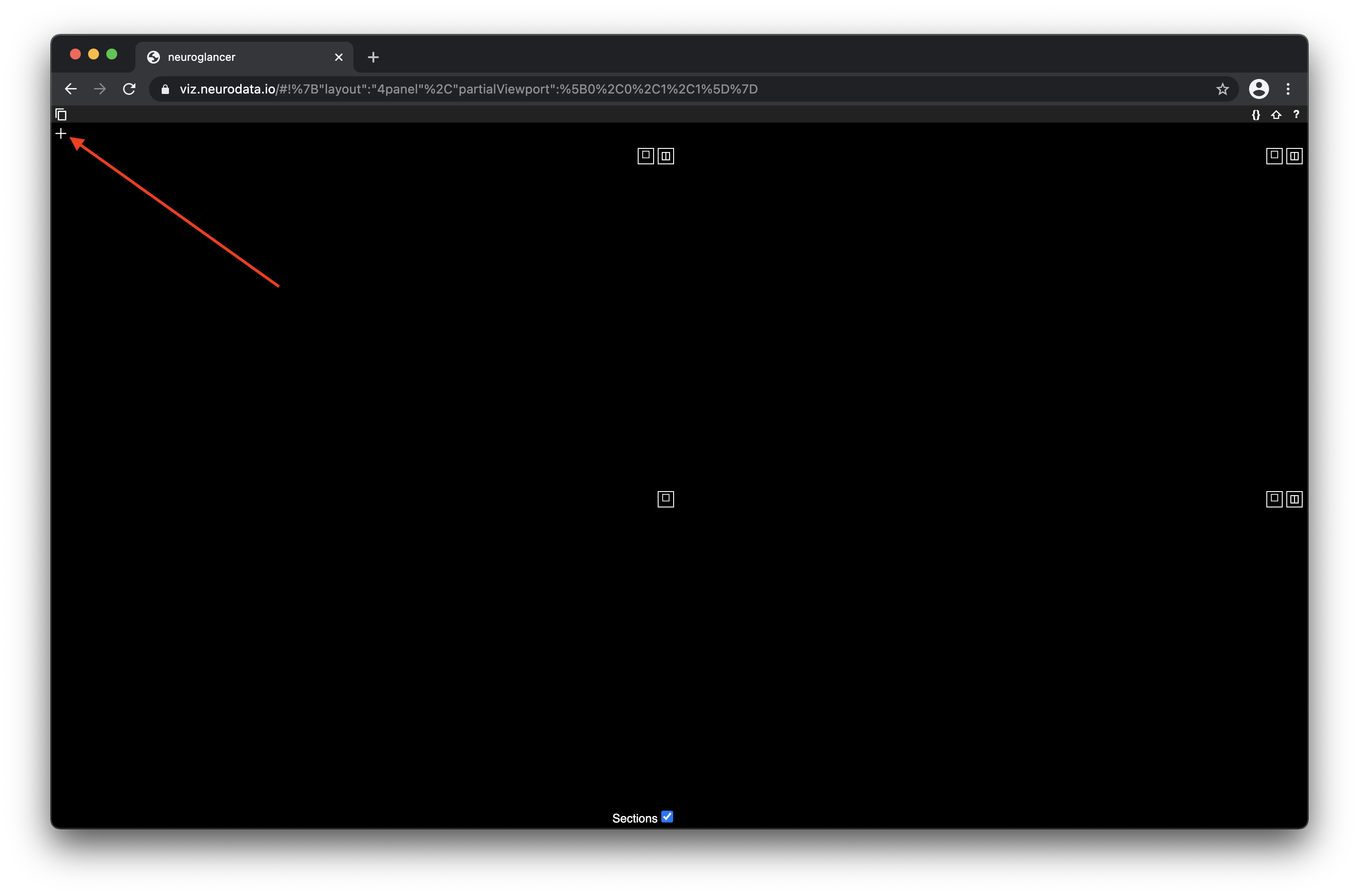
Go to https://viz.neurodata.io in a web browser.
Click on the ‘+’ on the top left of the Neuroglancer window (see image below).
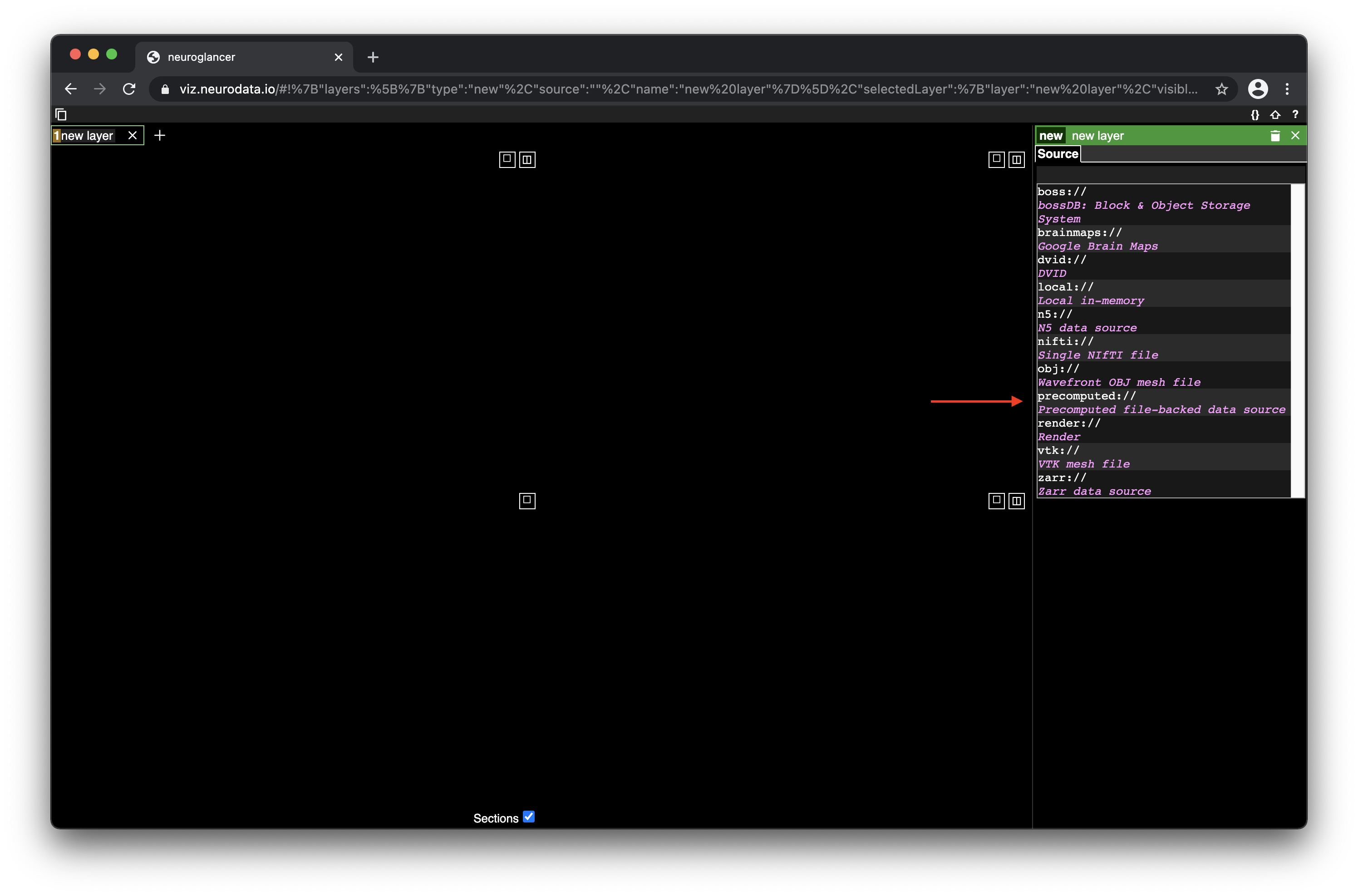
In the window that appears on the right side, choose precomputed from the drop-down menu (see image below).
After ‘precomputed://’ type the S3 path to the image layer (same as output_s3_path in preprocessing step above).

If you have CloudFront set up, you can replace the ‘s3://’ with your cloudfront domain name.
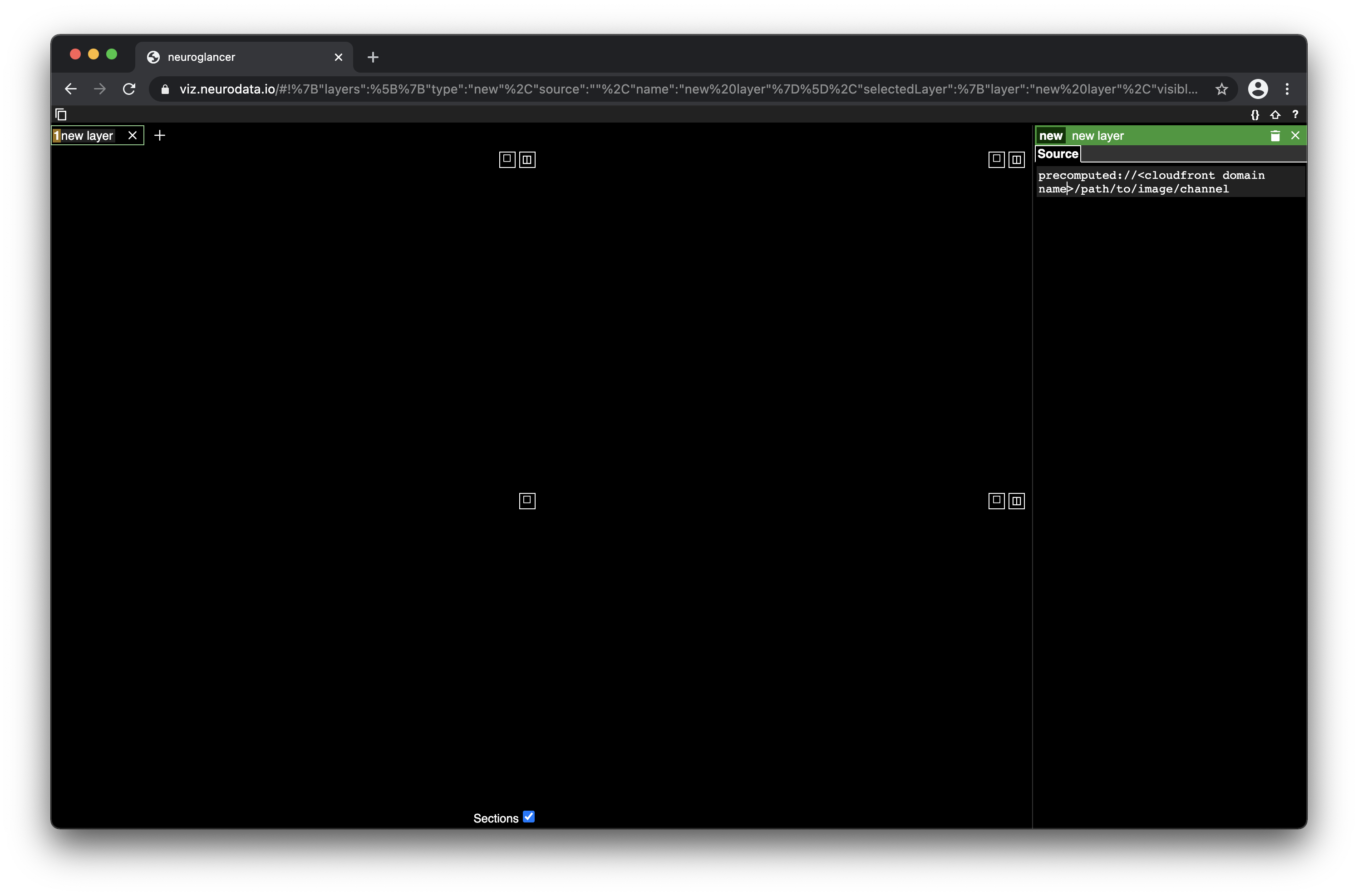
Hit enter and click “Create Image Layer” in the botom right of the Neurglancer window.

The data should start to load in 3 of the 4 quadrants. The bottom left quadrant is a 3D view of slices.
Hit ‘h’ while in a Neuroglancer window to view the help window.
Local
Once you have followed all instructions on the local setup page we can begin using CloudReg.
Currently the local pipeline can create precomputed volumes for visualization and perform registration. Additional scripts are available and can be found in references.
Convert 2D image series to precomputed format
Make sure Docker is open and running
Open a new Terminal window
Start the local CloudReg Docker image in interactive mode. Replace the below parameters between “<>” with your own. Run:
docker run --rm -v <path/to/input/data>:/data/input -v <path/to/output/data>:/data/output -ti neurodata/cloudreg:local
Once the previous command finishes, run:
python -m cloudreg.scripts.create_precomputed_volume /data/input file:///data/output <voxel_size e.g. 1.0 1.0 1.0>
Where the only required input is the voxel size of the images in microns. Replace the above parameters between “<>” with your own. More information about the precomputed volume parameters
Registration
The following commands can be used to register two image volumes.
Open a new Terminal window.
Run:
python3 -m cloudreg.scripts.registration -input_s3_path file://</path/to/local/volume> --output_s3_path file://</path/to/local/volume> -log_s3_path file://</path/to/local/volume> -orientation RIP
More information on local registration parameters
Visualization
All visualization is enabled through Neurodata’s deployment of Neuroglancer We will use a script to serve local data for visualization with our deployment of Neuroglancer.
Open a new Terminal window.
Start the local CloudReg Docker image in interactive mode. Replace the below parameters between “<>” with your own. Run:
docker run --rm -v <path/to/precomputed/data>:/data/input -p 8887:8887 -p 9000:9000 -ti neurodata/cloudreg:local
Run:
cd ../neuroglancer; python cors_webserver.py -d /data/input/
Now, in Google Chrome, go to https://viz.neurodata.io
Click on the ‘+’ on the top left of the Neuroglancer window (see image below).
In the window that appears on the right side, choose precomputed from the drop-down menu (see image below).
7. After ‘precomputed://’ type the local path to the image layer preceded by ‘http://localhost:9000’ (same as output_s3_path in create precomputed volume step above).  9. Hit enter and click “Create Image Layer” in the botom right of the Neurglancer window.
10. The data should start to load in 3 of the 4 quadrants. The bottom left quadrant is a 3D view of slices.
9. Hit enter and click “Create Image Layer” in the botom right of the Neurglancer window.
10. The data should start to load in 3 of the 4 quadrants. The bottom left quadrant is a 3D view of slices.
Hit ‘h’ while in a Neuroglancer window to view the help window.